Bin Sort

Assume that

1. the keys of the items that we wish to sort lie in a small fixed range and
2. that there is only one item with each value of the key.

Then we can sort with the following procedure:

1. Set up an array of "bins" - one for each value of the key - in order,
2. Examine each item and use the value of the key to place it in the appropriate bin.

Now our collection is sorted and it only took n operations, so this is an O(n) operation. However, note that it will only work under very restricted conditions.

By: sutha On 7:19 AM

Continue Reading

Solve the given equations using Stack(Post fix Notation)

Steps:
1. Read the equation as a string.
2.first pop two operand from the equation
3.If the third character is an operator we do the calculate the value for that operator and the operands.
4.Then push the calculated value in to the stack.
5.finally print the final value.


Implementation

By: sutha On 9:05 PM

Continue Reading

Decimal to binary Representaion using stack

Steps;

1.Read the decimal number.
2.Divide the decimal number until get zero
3.Find the remainder from rem= dec%2.
4.Push the remainder values int to the stack
6.Then pop the values from the stack until the stack become empty.


Implementation

By: sutha On 8:28 PM

Continue Reading

Selection Sort

Selection Sort

Selection sort is among the simplest of sorting techniques and it work very well for small files. Furthermore, despite its evident "naïve approach "Selection sort has a quite important application because each item is actually moved at most once, Section sort is a method of choice for sorting files with very large objects (records) and small keys. Algorithm 

Selection Sort(int []A)

1. for i=0 to n
2.         k=i
3.                for j=i+1 to n 
4.                    if(A[j]<A[i])
5.                        k=j
6.                    end if
7.                end for
8.            swap A[i,k]
9.  end for 

The worst case occurs if the array is already sorted in descending order. Nonetheless, the time require by selection sort algorithm is not very sensitive to the original order of the array to be sorted: the test "if A[j] < min x" is executed exactly the same number of times in every case. The variation in time is only due to the number of times the "then" part (i.e., min j ← j; min x ← A[j] of this test are executed.
The Selection sort spends most of its time trying to find the minimum element in the "unsorted" part of the array. It clearly shows the similarity between Selection sort and Bubble sort. Bubble sort "selects" the maximum remaining elements at each stage, but wastes some effort imparting some order to "unsorted" part of the array. Selection sort is quadratic in both the worst and the average case, and requires no extra memory.

For each i from 1 to n - 1, there is one exchange and n - i comparisons, so there is a total of n -1 exchanges and (n -1) + (n -2) + . . . + 2 + 1 = n(n -1)/2 comparisons. These observations hold no matter what the input data is. In the worst case, this could be quadratic, but in the average case, this quantity is O(n log n). It implies that the running time of Selection sort is quite insensitive to the input.

Implementation

 
output is:
 

       

By: sutha On 10:40 PM

Continue Reading

Parenthesis Matching using stack

Problem is given a string of parenthesis ‘(‘ and ‘)’ ,'{' and '}' , '[' and ']'  find out if there are matching pairs or not, typically this known as parenthesis matching problem.

For example : ‘((()))’ input will return TRUE, but ‘)(())’ will return FALSE.

By: sutha On 9:05 PM

Continue Reading

Bubble Sort

Bubble Sort

Bubble Sort is an elementary sorting algorithm. It works by repeatedly exchanging adjacent elements, if necessary. When no exchanges are required, the file is sorted.

SEQUENTIAL BUBBLESORT (A)

for i ← 1 to length [A] do
    for j ← length [A] downto i +1 do
        If A[A] < A[j-1] then
            Exchange A[j] ↔ A[j-1]

By: sutha On 10:40 PM

Continue Reading



Insertion Sort

If the first few objects are already sorted, an unsorted object can be inserted in the sorted set in proper place. This is called insertion sort. An algorithm consider the elements one at a time, inserting each in its suitable place among those already considered (keeping them sorted). Insertion sort is an example of an incremental algorithm; it builds the sorted sequence one number at a time. This is perhaps the simplest example of the incremental insertion technique, where we build up a complicated structure on n items by first building it on n − 1 items and then making the necessary changes to fix things in adding the last item. The given sequences are typically stored in arrays. We also refer the numbers as keys. Along with each key may be additional information, known as satellite data. [Note that "satellite data" does not necessarily come from satellite!]

Algorithm: Insertion Sort

It works the way you might sort a hand of playing cards:

1. We start with an empty left hand [sorted array] and the cards face down on the table [unsorted array].
2. Then remove one card [key] at a time from the table [unsorted array], and insert it into the correct position in the left hand [sorted array].
3. To find the correct position for the card, we compare it with each of the cards already in the hand, from right to left.

By: sutha On 10:39 PM

Continue Reading

Heap Sort

Heap Sort


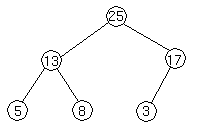
The binary heap data structures is an array that can be viewed as a complete binary tree. Each node of the binary tree corresponds to an element of the array. The array is completely filled on all levels except possibly lowest.

We represent heaps in level order, going from left to right. The array corresponding to the heap above is [25, 13, 17, 5, 8, 3].

The root of the tree A[1] and given index i of a node, the indices of its parent, left child and right child can be computed
 

PARENT (i)
        return floor(i/2)
LEFT (i)
        return 2i
RIGHT (i)
        return 2i + 1

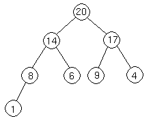
Let's try these out on a heap to make sure we believe they are correct. Take this heap,

which is represented by the array [20, 14, 17, 8, 6, 9, 4, 1].
We'll go from the 20 to the 6 first. The index of the 20 is 1. To find the index of the left child, we calculate 1 * 2 = 2. This takes us (correctly) to the 14. Now, we go right, so we calculate 2 * 2 + 1 = 5. This takes us (again, correctly) to the 6.
Now let's try going from the 4 to the 20. 4's index is 7. We want to go to the parent, so we calculate 7 / 2 = 3, which takes us to the 17. Now, to get 17's parent, we calculate 3 / 2 = 1, which takes us to the 20.

 

By: sutha On 10:34 PM

Continue Reading

Merge Sort

Merge Sort

Merge sort is based on the divide-and-conquer paradigm. Its worst-case running time has a lower order of growth than insertion sort. Since we are dealing with subproblems, we state each subproblem as sorting a subarray A[p .. r]. Initially, p = 1 and r = n, but these values change as we recurse through subproblems.

To sort A[p .. r]:

1. Divide Step

If a given array A has zero or one element, simply return; it is already sorted. Otherwise, split A[p .. r] into two subarrays A[p .. q] and A[q + 1 .. r], each containing about half of the elements of A[p .. r]. That is, q is the halfway point of A[p .. r].

2. Conquer Step

Conquer by recursively sorting the two subarrays A[p .. q] and A[q + 1 .. r].

3. Combine Step

Combine the elements back in A[p .. r] by merging the two sorted subarrays A[p .. q] and A[q + 1 .. r] into a sorted sequence. To accomplish this step, we will define a procedure MERGE (A, p, q, r).

Note that the recursion bottoms out when the subarray has just one element, so that it is trivially sorted.

By: sutha On 10:26 PM

Continue Reading